40%
30%
20%
10%
If all probabilities were equal (11%)
Almost half of all numbers will either start with a one or two.
This is a story about how numbers in the wild follow certain unexpected patterns. To start off, let me ask you this: if I were to give you this dataset of , how often would you expect the leading digit in the populations column to be a 2?
Would your answer change if I asked the same about those starting with a 9? There shouldn't be any reason why the leading digit wouldn't be random, so all 9 digits should be equally common right? Except when we chart the leading digits, we get the following:
So the leading digits are more focused around the smaller values and drop off as we go further out. This could be a one off result, so let's try again with another dataset. This time we're looking at electricity from natural gas
Once more the first digits in the dataset are biased towards a certain digit. The thing is that if we look at a couple more datasets, you will find similar behaviour. The fact that the numbers are more likely to have a certain leading digit isn’t very surprising - sometimes numbers can fall into ranges which have the same leading digit or sometimes it's just a quirk of how they are recorded. What is surprising however, is that however many datasets you look at…
1
2
3
4
5
6
7
8
9
1
2
3
4
5
6
7
8
9
1
2
3
4
5
6
7
8
9
1
2
3
4
5
6
7
8
9
1
2
3
4
5
6
7
8
9
1
2
3
4
5
6
7
8
9
1
2
3
4
5
6
7
8
9
1
2
3
4
5
6
7
8
9
1
2
3
4
5
6
7
8
9
1
2
3
4
5
6
7
8
9
1
2
3
4
5
6
7
8
9
1
2
3
4
5
6
7
8
9
1
2
3
4
5
6
7
8
9
1
2
3
4
5
6
7
8
9
1
2
3
4
5
6
7
8
9
1
2
3
4
5
6
7
8
9
1
2
3
4
5
6
7
8
9
1
2
3
4
5
6
7
8
9
1
2
3
4
5
6
7
8
9
1
2
3
4
5
6
7
8
9
1
2
3
4
5
6
7
8
9
1
2
3
4
5
6
7
8
9
1
2
3
4
5
6
7
8
9
1
2
3
4
5
6
7
8
9
1
2
3
4
5
6
7
8
9
1
2
3
4
5
6
7
8
9
1
2
3
4
5
6
7
8
9
1
2
3
4
5
6
7
8
9
1
2
3
4
5
6
7
8
9
1
2
3
4
5
6
7
8
9
An exploration of how real-world data often deviates from randomness.
So what is Benford's Law and how does it magically govern the distributions of datasets in the wild? The basic principle of this law is that the leading digit of numbers in a dataset are more frequently going to be small.
“How frequently”, you ask? Well Benford's Law puts the probability of a leading digit as:
P(d) = log10(d + 1) − log10(d)
where d is the leading digit we want to find the probability of. So essentially this boils down to the difference between the logarithm of the next digit and that of the current digit.
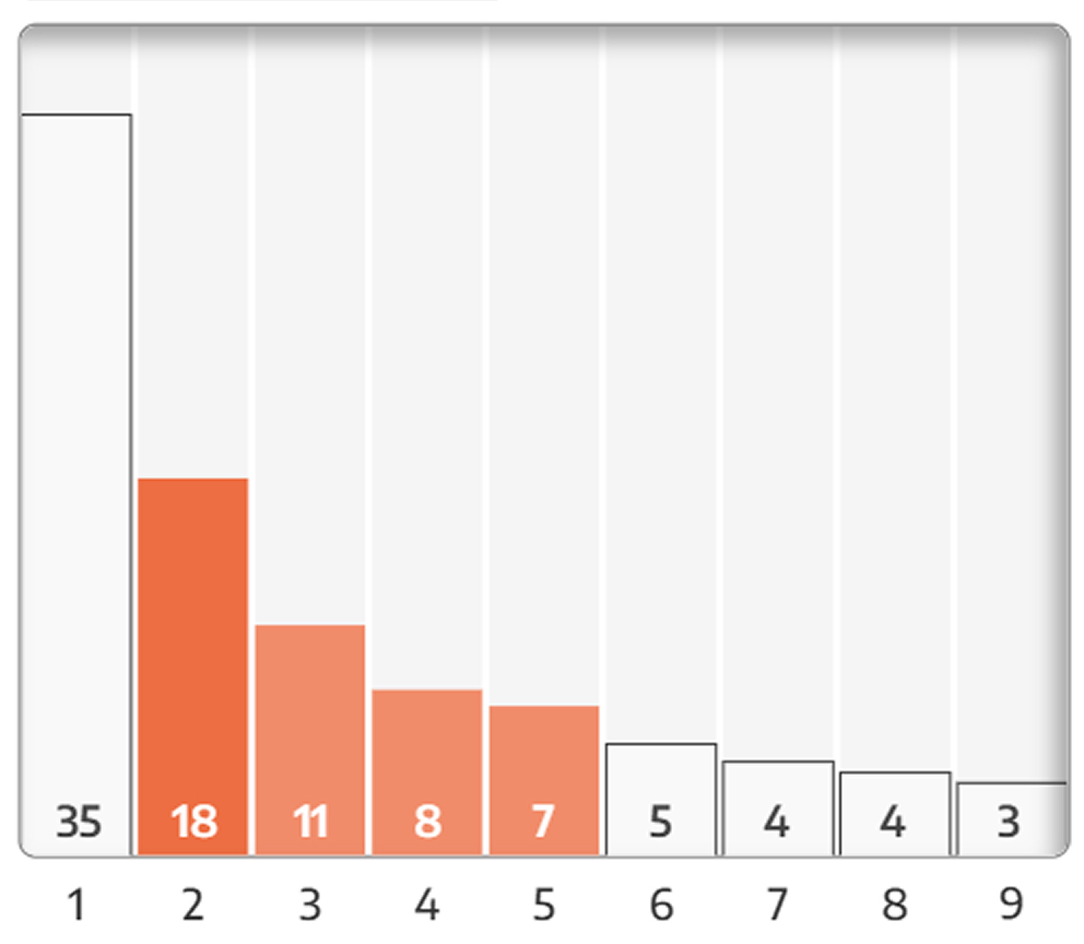
When graphed, this formula produces the following distribution:
In a distribution of naturally occurring values, the leading digit is more likely to be a smaller digit.
Almost half of all numbers will either start with a one or two.
In an even distribution we would expect each to have a probability of 11.11%, but in practice Benford's law puts the odds of a leading digit of 1 to be 30.1% - almost three times more likely! Additionally, you are more than 6 times more likely to find a leading digit of 1 than a 9!
There are several explanations for this, some more mathematically involved than the others. But I want to stick to a more intuitive explanation for Benford’s Law. Many real-world examples of Benford's Law are affected by multiplicative growth - e.g. money compounds, populations change exponentially with each generation, prices are influenced by a percentage of inflation, etc.
What we find in multiplicative growth is that the leading digit tends to stick around at lower values for a lot longer than digits on the higher end of the range. For example, suppose you deposit 100 dollars in a bank which gives you a good interest per year. This is what the next 100 years would look like.
As you can see, compounding by 5% generates a bunch of numbers starting with 1s, 2s but largely skips over the larger digits as the sequence progresses.
In case you haven't used a proportion plot before, here's a (not really) quick guide.
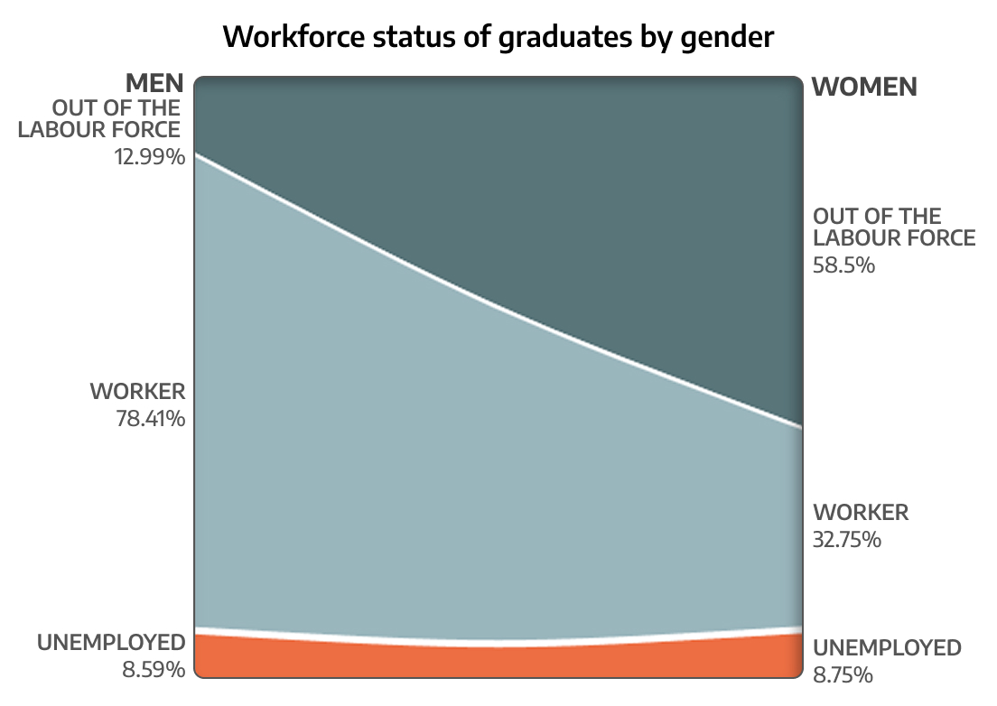
Proportion plots take a look at two different distributions and show how the same value deviates in different scenarios. The following chart shows the difference in women's representation in labour force vs men's.
Source: Periodic Labour Force Survey 2023-2024, National Sample Surveys, National Statistics Office via Data For India
The digits on the left are share of leading digits from our observed distribution, from 1 to 9.
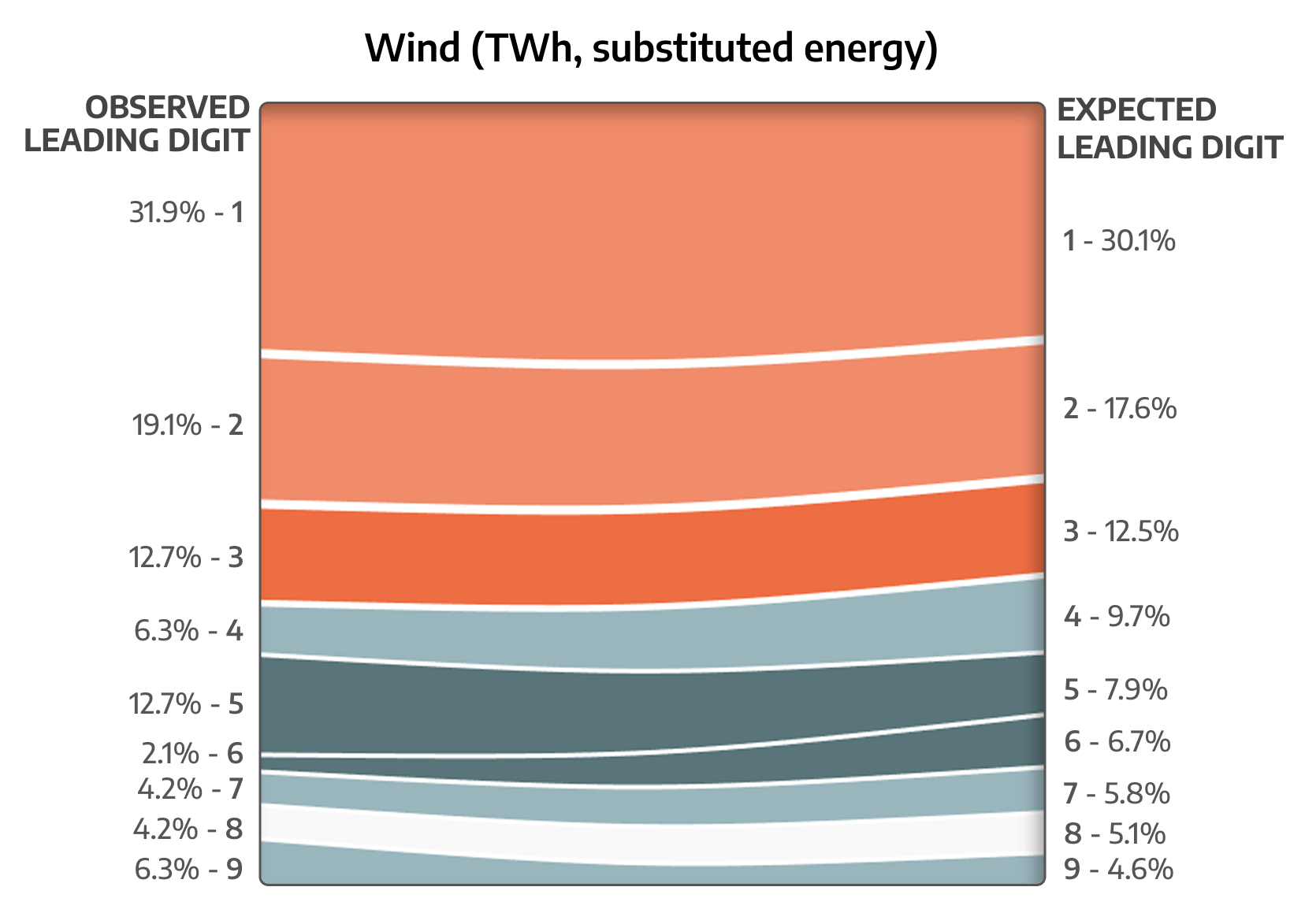
Those on the right are the expected proportion according to Benford’s Law.
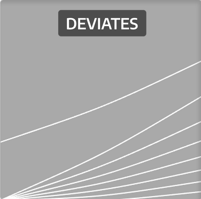
Sloping lines between the two sides indicates that there is some deviation from the expected behaviour.
If the distribution fits Benford’s Law you will see largely horizontal bands across the chart as opposed to heavily sloping bands when the two sides don't match.
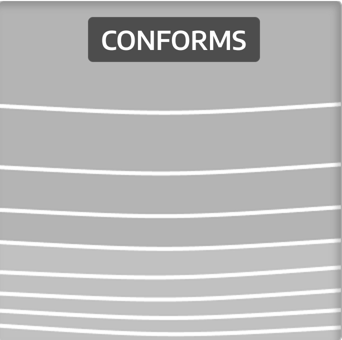
Often, colour will be used to denote how closely the band for a specific number lines up with it’s expected proportion.

You will see these labels throughout the course of the explainer.
I use the Mean Absolute Deviation (MAD) score to measure how close the distribution is to Benford’s distribution. While this is standard practice, it is still quite rigorous leading to many seemingly close results failing the test:
For example this falls under “Doesn’t conform”
While I will still show these results, I urge you to eyeball the chart and decide if you still feel that that the general takeaway of “smaller numbers are more likely” feels apt.
That said, in quite a few cases it easier to spot benford's patterns with a standard bar chart, which is why you can toggle between it and the proportion plot here and in the navbar below.
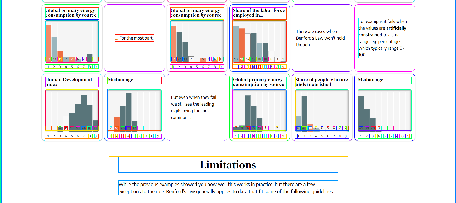
Let's see how Benford's Law plays out in the wild. It's not just numbers in datasets that conform to Benford's Law, but we will start there.
Let's take a closer look at some of the columns we looked at in previous sections. While most seem to fit the bill we also notice a couple patterns among those that don't quite follow Benford's Law. We will dive deeper into those in a later section though.
1
2
3
4
5
6
7
8
9
1
2
3
4
5
6
7
8
9
1
2
3
4
5
6
7
8
9
For a random selection I used all of the datasets featured on OWID's data page
1
2
3
4
5
6
7
8
9
1
2
3
4
5
6
7
8
9
1
2
3
4
5
6
7
8
9
1
2
3
4
5
6
7
8
9
1
2
3
4
5
6
7
8
9
1
2
3
4
5
6
7
8
9
Despite the wide range of topics, we see that most exhibit Benford's Law
1
2
3
4
5
6
7
8
9
1
2
3
4
5
6
7
8
9
... For the most part.
1
2
3
4
5
6
7
8
9
1
2
3
4
5
6
7
8
9
There are cases where Benford's Law won't hold though
For example, it fails when the values are artificially constrained to a small range. eg. percentages, which typically range 0-100
1
2
3
4
5
6
7
8
9
1
2
3
4
5
6
7
8
9
But even when they fail, we still see smaller leading digits being more common...
1
2
3
4
5
6
7
8
9
1
2
3
4
5
6
7
8
9
1
2
3
4
5
6
7
8
9
At its core, everything on the web is just a bunch of tiny rectangles styled and rearranged together to form the content you see on a daily basis. I wrote a bit of code that would go through every HTML element on this page and create a dataset of all their areas. This is what we get when we analyse these areas.
HTML elements with their boundary boxes highlighted
I have a pile of old National Geographic magazines that I like to flip through from time to time. I decided to pick one up and record every number I could find. This lead to me spending an hour logging and categorizing numbers from National Geographic's October 2010 issue before I ended up with a set of 239 valid numbers.
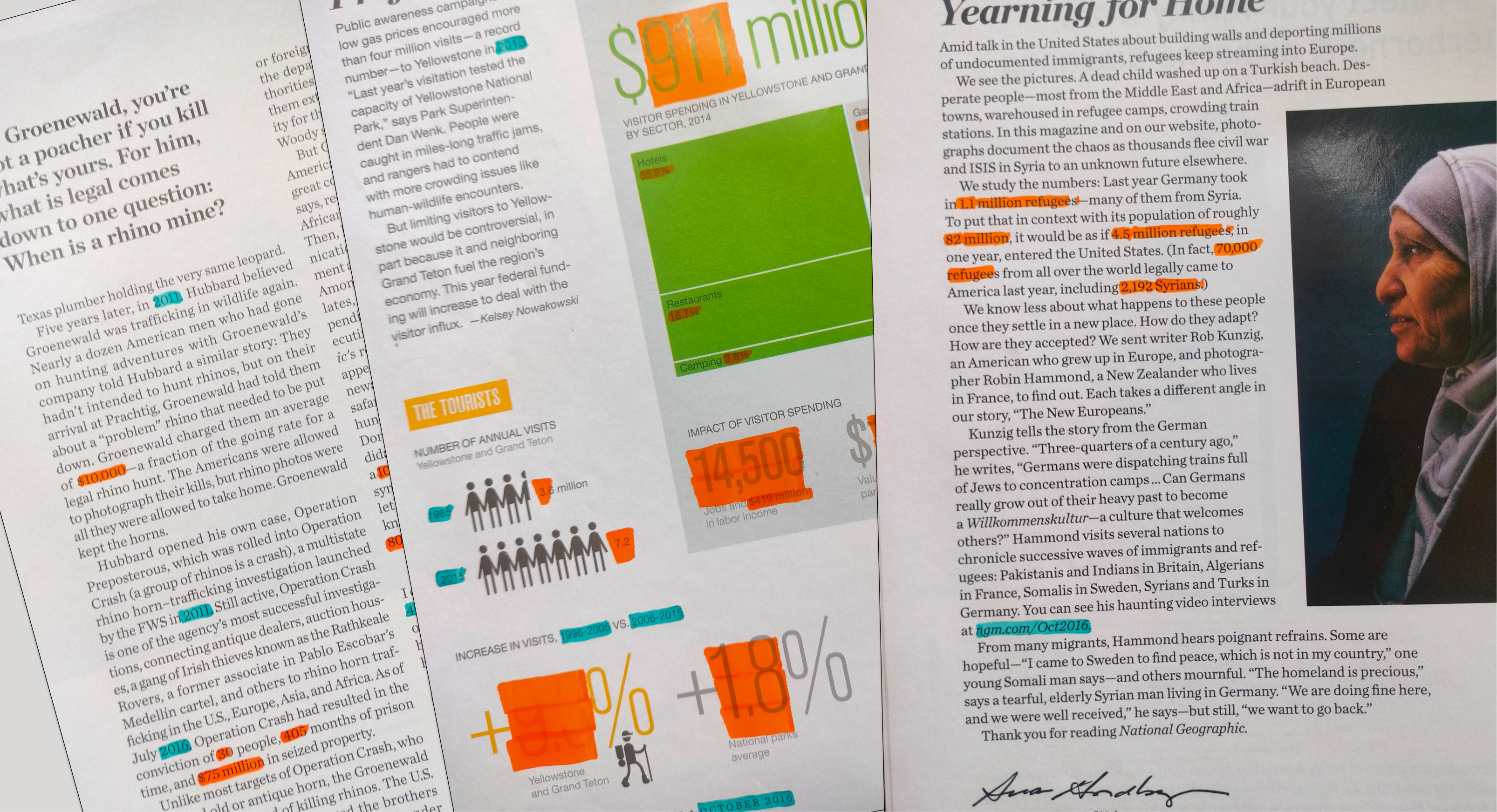
Categorized pages from National Geographic's October 2010 issue
The numbers excluded from this set include assigned values like page numbers, phone numbers, address markers, dates and years. Note that while normally values like percentages are problematic for Benford's Law since they have a limited range (0-100), in this case since we are lumping them in with different types of numbers of varying scales, this constraint is a lot less of a concern. Finally, when charted these are the results:
Where Benford's Law starts to fall apart
While the previous examples showed you how well this works in practice, there are a few exceptions to the rule. Jim Frost has a great writeup on this if you want to dive deeper.
Phone numbers in a state wouldn’t follow Benford’s law because being an assigned, they would simply run down their list of available numbers, each being assigned with equal probabilities. Additionally they may even have a fixed area code as the prefix, further throwing off the leading digit distribution.
Another requirement is that the numerical values should span several ranges of magnitude. A good rule of thumb is that it should span at least 3 ranges of magnitude (eg. 1 to 1000 ie, 10^0 to 10^3) - in general the more orders of magnitude, the more pronounced the effect is.
So year columns suck for Benford's Law. Not only is it an assigned number, it even has one of the smallest ranges of magnitude (2025 and 1900 are in the same order of magnitude, i.e. the thousands). As such here are some year columns pulled from Our World in Data's datasets to illustrate this point.
1
2
3
4
5
6
7
8
9
1
2
3
4
5
6
7
8
9
1
2
3
4
5
6
7
8
9
1
2
3
4
5
6
7
8
9
1
2
3
4
5
6
7
8
9
... Yup, not great.
1
2
3
4
5
6
7
8
9
1
2
3
4
5
6
7
8
9
1
2
3
4
5
6
7
8
9
1
2
3
4
5
6
7
8
9
1
2
3
4
5
6
7
8
9
1
2
3
4
5
6
7
8
9
1
2
3
4
5
6
7
8
9
1
2
3
4
5
6
7
8
9
1
2
3
4
5
6
7
8
9
The dataset should be generated from a natural process. If it is restricted or forced to fit into a specific size or cutoff, it fails to follow Benford's Law. For example, the UN's Human Development Index measures a country's development on a scale from 0 to 1. Because of this artificial restriction, the leading digits do not follow Benfords
Because when do they not. But yes, larger datasets tend to provide a more accurate representation of Benford's Law.
Naturally occurring datasets which fit the above criteria can be expected to have their first digits follow Benford’s Law. The key word being “naturally occurring” here - fabricated or randomly generated data will often not follow this principle.
This leads to it often being applied in fraud detection. From fake election data to accounting fraud, Benford’s Law is applied by testing the first digits of the data.
Remember that while it is helpful, this is by no means a sure way to detect manipulation, it is merely indicative of foul play.
The Data: The bulk of the data was used from Our World in Data and their Grapher Chart API. For a random selection of datasets, I used a python script to select featured datasets on OWID's data page and then pull in the actual data via their API. In total 139 columns, from 41 datasets were analysed and charted in some capacity throughout the project. The proportion plot example uses data from National Sample Surveys, National Statistics Office via Data For India.
Benford's Law Analysis: Every column in the previous collection was tested for Benford's Law on both its first digits and last digits (although this was not included in the explainer). To mathematically test how close the data was to Benford's expected distribution, I used the Chi-Squared Goodness of Fit test. However due to large sample sizes in our datasets, the Chi-Squared test often indicated significant differences even when the distributions visually appeared close.
I then moved on to using Mean Absolute Deviation (MAD), with Nigrini's thresholds as a baseline for conformity. While this worked better than Chi-Squared, there were still quite a few datasets which looked close but had high MAD values. So I ultimately decided that while I will still show these results, I would also visualize each of the datasets and urge the reader to decide if "smaller leading digits do occur more frequently than larger ones".
Development: This explainer was built using Sveltekit. All of the code used to scrape and analyse the data are publicly available on GitHub. I am still in the process of cleaning up the codebase (said every dev ever...), but rest assured that all the frontend and analysis code is available there.
Also here's a link to the chart gallery for this page. Remember that you can toggle between chart types using the navbar.
AI Usage: In general I use coding Github Copilot as a coding assistant to speed through the boilerplate parts of the code and analysis. No LLMs were used in the writing of this text content or research and analysis.
P.S. I am by no means a statistics expert, I just get easily distracted by pointless math. If you spot any issues feel free to reach out to me on any of my socials listed below.
Schubert de Abreu | Personal site | BlueSky | Twitter | LinkedIn